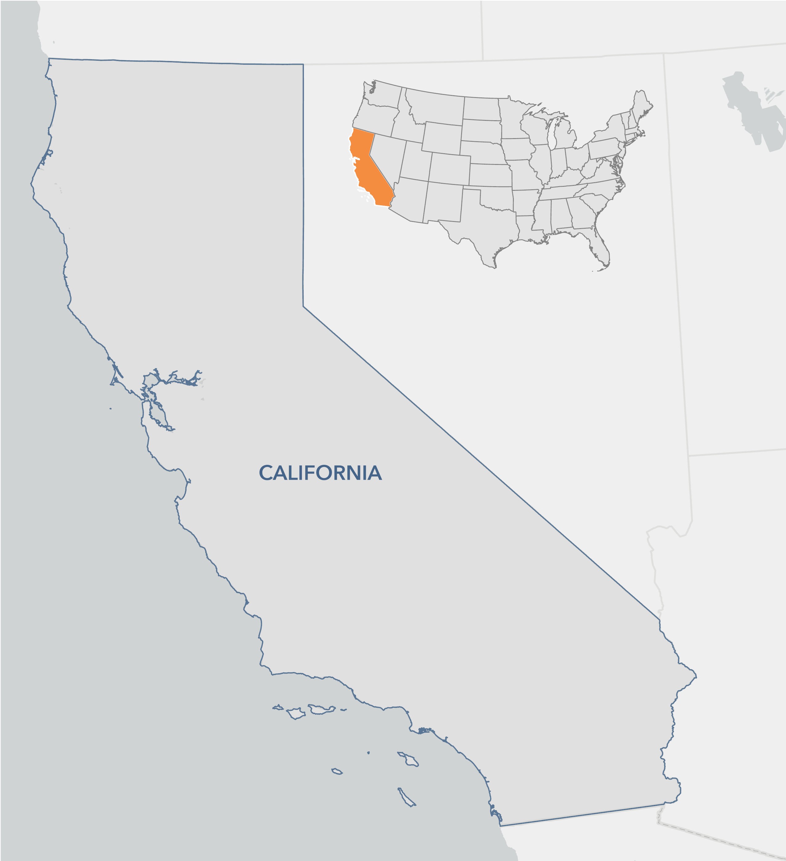
California
Structure Graph Data
Characterizing fire connectivity in the built environment
Wildfire is changing. Across the U.S. — and especially in the West — fires are becoming more frequent, more severe, and more capable of moving rapidly through communities.1,2 As development expands into fire-prone landscapes, the line between wildland and urban fire has blurred. Meeting this challenge requires better data, sharper tools, and a clearer understanding of how fire behaves once it reaches the built environment.3
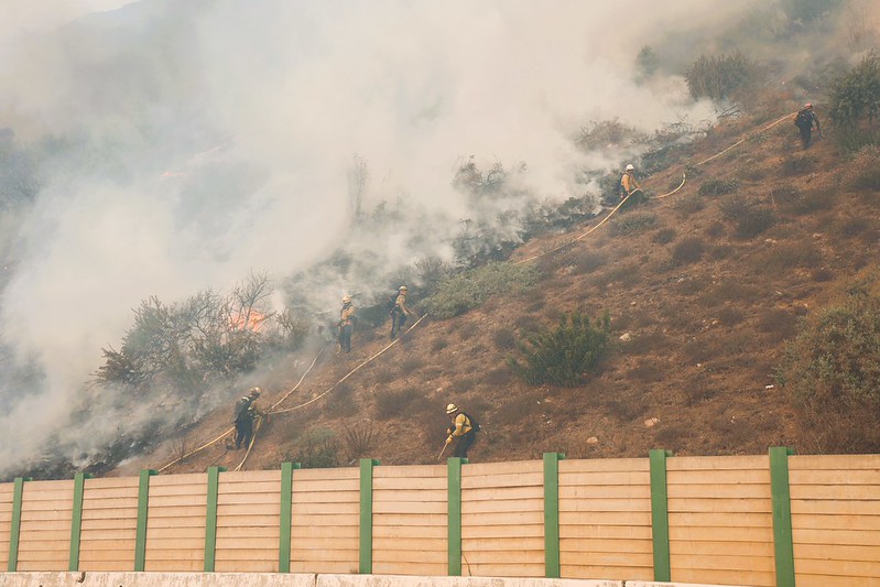
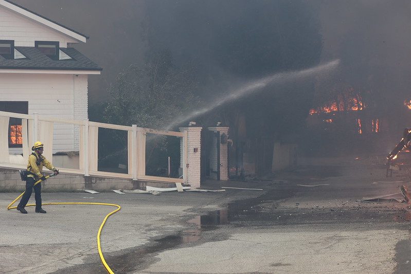
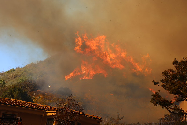
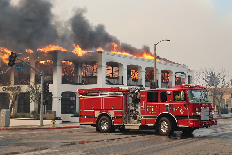
During the Palisades Fire in early 2025, flames advanced down a hillside toward homes in Los Angeles, illustrating the critical moment when wildland fire behavior intersects with the built environment. Photo © CAL FIRE.
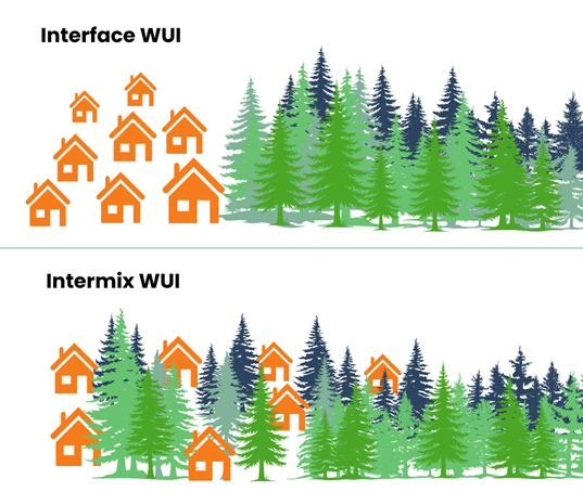
Two common WUI patterns—Interface and Intermix—show how the arrangement of homes relative to vegetation shapes the conditions under which wildland fire transitions into the built environment.
When flames reach the wildland edge, they don’t stop: the built environment itself becomes fuel.4 Structures, fences, and outbuildings can carry fire from structure to structure, creating chains of ignition long after the wildfire front has passed.
This dynamic is especially pronounced in the Wildland–Urban Interface (WUI), where homes sit close together in fire-prone landscapes. Traditional fuel-based risk models capture how fire reaches communities, but they rarely account for what happens once it arrives—how neighborhood design and structure density create pathways for fire to propagate from structure to structure.
To better understand this built-environment dynamic, Vibrant Planet built the California Structure Graph: a statewide dataset that maps how California’s 13.6 million structures relate to one another spatially and how those relationships shape the potential for fire to move from structure to structure. Using open building footprint data and a large-scale geospatial processing pipeline, the analysis transformed structure data into a network that reveals fire transmission pathways.
The dataset shows which buildings are positioned to act as transmission hubs if ignited and which neighborhoods have high-connectivity clusters where fire could propagate rapidly from structure to structure. This helps planners, fire scientists, and local agencies understand how neighborhood spatial patterns create exposure—not just wildland fuel proximity.
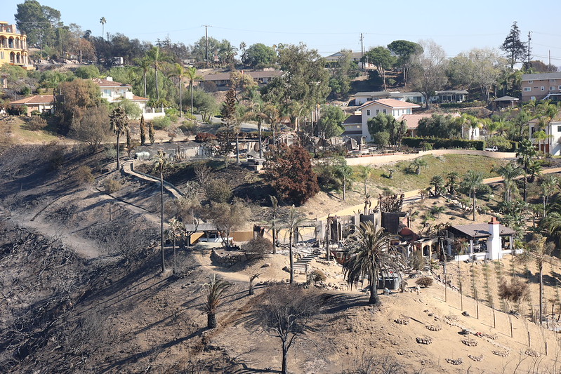
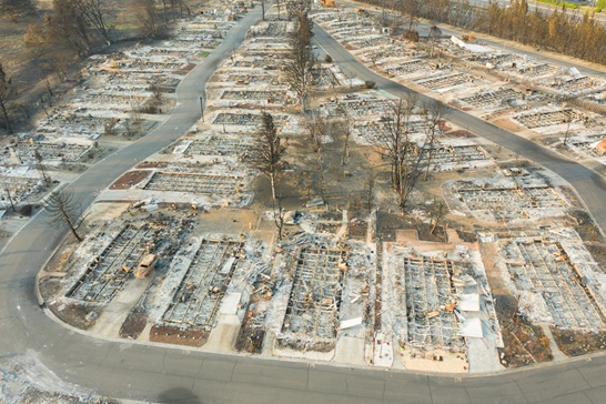
The 2024 Mountain Fire burned nearly 20,000 acres and destroyed 243 structures, including major losses in Camarillo Heights neighborhood shown here. Dense WUI neighborhoods like this illustrate how structure spacing can shape building-to-building fire spread. Photo © CAL FIRE.
An important caveat: this dataset is not a vulnerability score or a predictive model. It does not account for building materials, defensible space, or parcel-level conditions. It is an exposure layer—a transparent, open-source way to quantify how community form and building density create pathways for fire spread, complementing rather than replacing structure-level vulnerability assessments.
What is Structure Graph Data?
The California Structure Graph describes how structures are positioned relative to one another and how those spatial relationships create potential pathways for structure-to-structure fire spread. Rather than treating buildings as isolated features, the dataset preserves the distances between nearby structures so connectivity can be examined explicitly.
To do this, the built environment is represented as a network:
- Each building is treated as a node—whether a home, garage, shed, or commercial structure.
- A connection (edge) exists between two buildings when their footprints fall within a specified separation distance.
- Degree counts how many nearby buildings are connected to a given structure within a chosen distance range.
Together, these elements capture how tightly or loosely buildings are arranged within neighborhoods. A structure’s degree reflects how many other structures sit close enough to form potential exposure pathways—making degree a simple, interpretable measure of built-environment connectivity.5
Seen through this lens, the Structure Graph works much like a social network for buildings: structures with higher degree are more embedded in their surroundings and can act as local connectivity hubs if ignited, while isolated structures have few or no nearby neighbors and are less involved in structure-to-structure fire spread. How influential these connections are, however, depends on the distances at which they are evaluated—shifting the scale of analysis from immediate neighbors to entire neighborhoods.
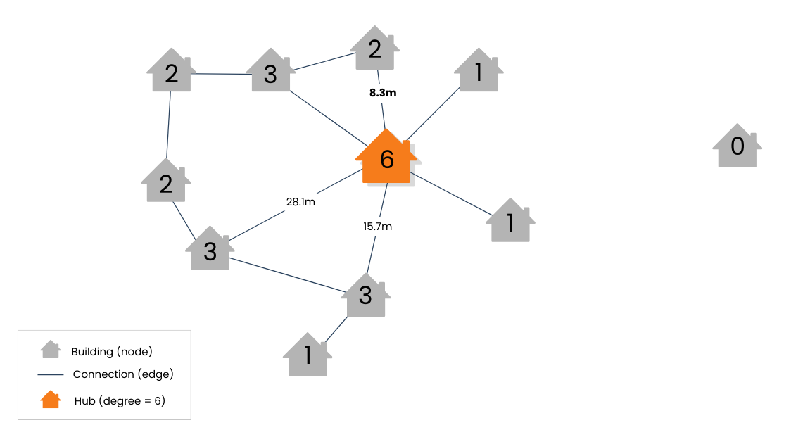
Structure connectivity graph: Numbers show degree, the count of neighboring structures within a chosen distance threshold. The highlighted structure (orange) is a local connectivity hub with six nearby neighbors, while the isolated structure (degree = 0) has no connections within the threshold. Graphic by Vibrant Planet Data Commons.
Tightly packed homes in Carmel-by-the-Sea demonstrate how structure spacing drives high connectivity at 10m, 50m, and 100m distance thresholds. Photo © Mac Gaither / Unsplash.
Distance Thresholds Define Exposure
Edges in the Structure Graph are defined using structure separation distance (SSD), measured as the minimum boundary-to-boundary distance between two structure footprints. The dataset includes all structure pairs within 100 meters, retaining the exact separation distance for each pair.
For scalability, these structure-to-structure relationships are distributed across edge layers partitioned by distance ranges (for example, 0–10 m, 10–50 m, and up to 95–100 m). The node layer, in contrast, summarizes each structure’s overall connectivity across the full ≤100 m network. Because distances are retained at the edge level, users can examine connectivity at any distance scale by filtering or aggregating edges—without reprocessing the underlying data.
Distance thresholds in the Structure Graph should be understood as analytical lenses, not fixed physical cutoffs. Because exact SSD’s are retained for every edge, users are not constrained to predefined bins or assumptions about fire behavior.
Short distances (≈10 m) emphasize immediate adjacency where direct flame contact or intense radiant heat may be plausible. Broader distances provide insight into near-neighborhood (≈50 m) and neighborhood-scale (≈100 m) connectivity patterns that shape how exposure could cascade once fire enters the built environment.
This design allows users to define distance thresholds appropriate to their modeling assumptions, local conditions, or research questions—without reprocessing the underlying data. Connectivity can be examined at fine scales, aggregated across broader neighborhoods, or filtered dynamically to support sensitivity testing and scenario comparison
Across California, these patterns vary widely. Some structures are effectively isolated even at neighborhood scales, while others are embedded within dense networks of nearby buildings. Viewed collectively, these differences reveal where tightly connected clusters and local connectivity hubs concentrate, supporting both local analysis and consistent regional comparison.
Note on distance and fire behavior: Structure-to-structure fire spread depends on many interacting factors, including wind speed and direction, fuel characteristics, building materials, and suppression actions. While research shows that direct flame contact, radiant heat, and ember exposure can occur across a wide range of distances under extreme conditions, no single distance threshold universally defines these processes. The Structure Graph is therefore designed as an exposure and connectivity framework, not a fire-behavior model.6, 7, 8
Geography & Scope
California’s combination of extreme fire weather and dense development in fire-prone landscapes makes it a critical setting for understanding how fire moves once it reaches the built environment. Wind-driven events, long dry seasons, and frequent human ignitions have produced some of the most destructive wildland–urban interface fires in modern history — including the 2017 Tubbs Fire, the 2018 Camp Fire, and the 2025 Eaton and Palisades Fires — where losses accelerated through structure-to-structure transmission inside neighborhoods.
The California Structure Graph captures this dynamic at full statewide scale. Built from Overture Maps Foundation building footprints current as of November 4, 2025, the dataset represents approximately 13.6 million structures across the entire state, from dense urban cores to rural foothill communities and coastal development zones. Mapping connectivity consistently across these varied settlement patterns allows communities and agencies to understand how neighborhood form influences potential fire transmission — and to compare exposure patterns across regions using a shared, transparent method.
By applying a single, reproducible approach statewide, this dataset provides both local-scale precision for mitigation planning and a foundation that can be extended to other fire-prone states using comparable open footprint data and processing methods.
Are you interested in exploring or applying this dataset in your work?
We want to hear from you!
Vibrant Planet and Vibrant Planet Data Commons are actively tracking how their datasets are used to support impactful wildfire management and research. Contact us to share your ideas, feedback, or success stories, and help us make data-driven solutions a reality.
Why This Dataset Matters
Science, Management, and Policy Applications
Wildfire risk is shaped not only by forests, fuels, and topography—but increasingly by the physical layout of our communities. In many destructive WUI fires, the built environment becomes part of the fuel complex, enabling fire to move rapidly from one structure to the next. Traditional wildfire models typically stop at the edge of town. Structure connectivity data fills this gap.
By representing every building as part of a spatial network, this dataset allows analysts and planners to understand how fire could move within communities once it arrives:
- Identify transmission points: Highly connected buildings (“hubs”) have many nearby neighbors and can act as ignition sources with outsized influence if they burn.
- Understand cascade potential: Dense clusters create conditions where a single building ignition can propagate sequential losses—a dynamic many wildfire models do not explicitly capture once fire enters the built environment.
- Target mitigation strategically: Home hardening, defensible space, and vegetation treatments can be placed to disrupt high-connectivity corridors, not just applied uniformly.
- Inform planning and development: Connectivity metrics help communities understand how setbacks, parcel patterns, and density influence future fire exposure.
This shifts the risk conversation from "Will fire reach this community?" to "How will fire move through this community once it arrives?", a perspective that is increasingly essential for modern risk assessment.
How the Structure Graph Was Built
The California Structure Graph is built in three steps: identifying structures, measuring separation distances, and counting connections.
Step 1: Identify structures using building footprints
The analysis begins with building footprint polygons, which include homes, garages, sheds, commercial buildings, and other structures. Because these are full structure footprints—not points—they allow precise, edge-to-edge measurements.
Why footprints matter: A warehouse that appears far from a home by centroid distance might be only five meters away at its nearest wall. Using footprints captures the distance fire would actually need to cross.
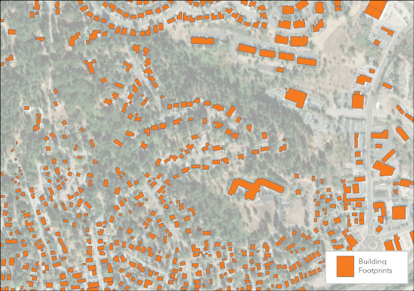
Example of Overture's open building footprints overlaying satellite imagery in a WUI community located in Northern California.
Step 2: Create edges using structure separation distance (SSD)
Edges represent pairs of structures separated by 100 meters or less, measured as the minimum boundary-to-boundary distance between their footprint polygons (SSD).
To generate these edges efficiently at statewide scale, the workflow first builds a spatial index by assigning each structure to 100 m by 100 m tiles based on the extent of a 50 m buffer around its footprint. Structures that share a tile are treated as candidate neighbors. Candidate pairs are then filtered using a geometric proximity test: pairs are retained only when the two 50 m buffered footprints intersect, ensuring the structures are within 100 m of each other.
For each retained pair, the workflow computes and stores the exact SSD (ST_Distance between polygons). A centroid-to-centroid line geometry is also generated for visualization, and edges are exported in distance ranges (for example, 0–10 m, 10–50 m, and up to 95–100 m) to support scalable use.
The result: A dataset containing every structure pair in California separated by 100 meters or less, with exact distances recorded.
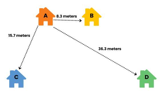
Example of structure separation distances used to build the California Structure Graph. Each pair of buildings within 100 meters becomes an edge in the graph, with the exact boundary-to-boundary distance recorded. These measurements (e.g., 8.3 m, 15.7 m, 36.3 m) form the basis for the connectivity metrics calculated statewide.
Step 3: Summarize connectivity on nodes
After edges are created, the workflow summarizes local connectivity for each structure (node). The degree is calculated as the number of edges connected to each node within the ≤100 m network. The workflow also computes ego-network statistics including clustering coefficient, along with summary distance metrics (minimum and mean SSD) derived from each structure’s connected edges.

Summarizing connectivity at the structure level. A local structure network shows how edge-level separation distances are aggregated into node-level metrics, including degree, clustering, and summary structure separation distances (SSD), describing how an individual structure is embedded within its immediate neighborhood.
Applications
Fire Science & Risk Modeling
The analysis starts by using open building polygons which include homes, garages, sheds, commercial buildings, and other structures. Because these are full building footprints—not points—they allow precise, edge-to-edge measurements.
- Improving predictive models: Including metrics like structure separation distance and centrality can improve predictions of structure loss by capturing transmission pathways that traditional fuel-based models miss.
- Enhance WUI mapping: Connectivity metrics clarify not just where vegetation and buildings meet, but how building-to-building exposure amplifies risk—supporting refined WUI classifications and more accurate community exposure baselines.
Landscape & Home Mitigation
- Disrupt destructive fire corridors: By identifying clusters of highly connected structures—or “fire corridors”—managers can place vegetation treatments, fuel breaks, or targeted home-hardening measures where they will disrupt transmission pathways most effectively.
- Target neighborhood-scale mitigation: Connectivity highlights high-leverage clusters where protecting a few structures reduces risk for many, helping communities direct limited resources where they provide the biggest network-wide benefit.
Planning, Development, and Rebuilding
- Support risk-informed land-use decisions: Connectivity and centrality metrics can inform subdivision design, zoning decisions, rebuild standards, and development planning by quantifying how setbacks, density, and parcel layout influence future fire exposure.
- Guide safer rebuilds after fire: When recovery begins, structure networks can help planners understand how pre-fire neighborhood form contributed to losses—and where future development standards can reduce exposure.
Insurance, Policy, and Governance
- Inform insurance pricing and incentives: Understanding potential structure-to-structure spread supports more transparent risk categorization and can help insurers design incentives for reducing neighborhood-scale exposure.
- Shape codes and community standards: Connectivity analysis can provide evidence for updating building codes, hardening requirements, defensible space regulations, and neighborhood-scale mitigation standards.
Emergency Response & Preparedness
- Understand potential for rapid structure spread: Fire departments can use connectivity patterns to identify where structure-to-structure ignition may accelerate, supporting decisions about pre-positioning resources and prioritizing evacuations.
- Identify gaps in response capability: Where extremely high connectivity coincides with limited staffing, water supply, or egress capacity, departments can highlight urgent needs for investment or planning upgrades.
Applied Use Case: Nevada County, California
Nevada County is consistently ranked among the highest wildfire-risk counties in the United States.10 Much of that risk comes from wildland fire exposure along the edges of communities. But what happens after a fire reaches the built environment depends on something traditional models rarely capture: how homes are arranged, how close they sit to one another, and how those spatial relationships can accelerate structure-to-structure fire spread.
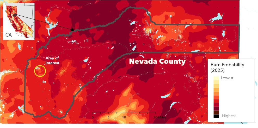
Burn probability across Nevada County. Burn probability (BP) reflects the annual likelihood that wildfire will burn a given location. Higher BP values occur along the center and northeastern portions of the county, where topography, vegetation, and historical ignition patterns coincide.
Structure Graph data allows us to see and integrate those dynamics more clearly. The maps and figures that follow are derived from an applied analysis that combines the California Structure Graph with wildland burn probability and exposure data. This Nevada County example demonstrates how structure connectivity metrics can be layered onto existing risk information to explore neighborhood-scale exposure pathways and modeled loss outcomes.
Where wildland exposure meets built-environment connectivity
We can begin to see these dynamics as we zoom in to larger scales. Take for example, zooming in to a neighborhood outside Grass Valley, California as shown in Figure 1. The outer edges show the highest wildland burn probability—no surprise there, as it’s closest to dense, wooded areas. What the structure graph adds is the ability to see how those edge homes are directly connected to interior homes through dense 10-meter networks. In other words, the fate of “interior” structures is tightly linked to what happens along the perimeter. Once wind-driven flame or radiant heat ignites a home on the edge, exposure can cascade inward through these tight clusters.
This is a pattern seen repeatedly in destructive WUI fires, including the Eaton and Palisades Fires of 202511,12: the first homes to ignite rarely remain the only ones affected.
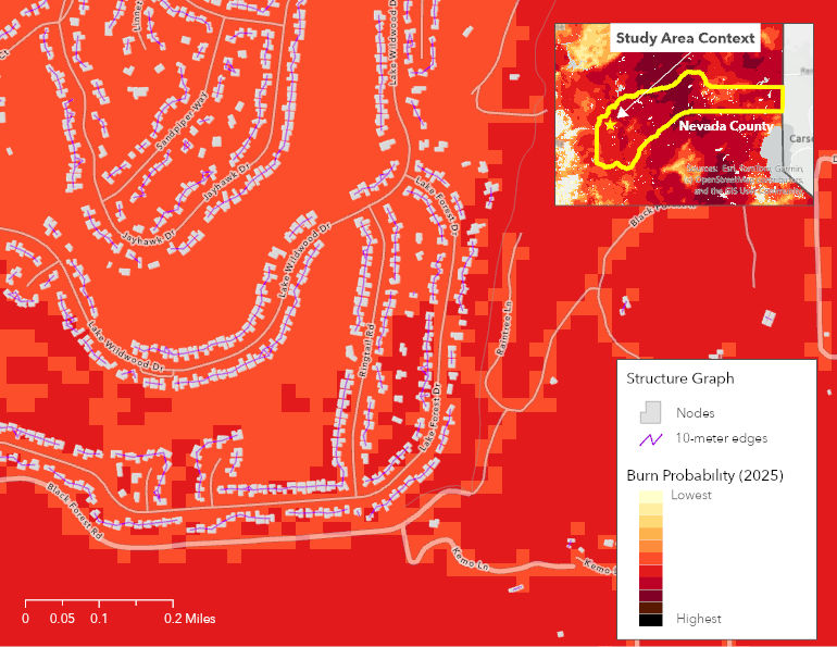
Figure 1. Neighborhood-scale burn probability and structure graph connectivity. Within this Nevada County neighborhood, burn probability is highest along the wildland-facing edge and decreases toward the interior. The 10-meter structure graph highlights where homes are spaced close enough for radiant heat or flame contact to be physically possible if a structure ignites. While burn probability indicates where wildfire is most likely to approach from the surrounding landscape, the structure graph provides insight into how the built environment may influence potential exposure pathways once fire reaches the community. Map by Vibrant Planet Data Commons
Clusters that rise and fall together
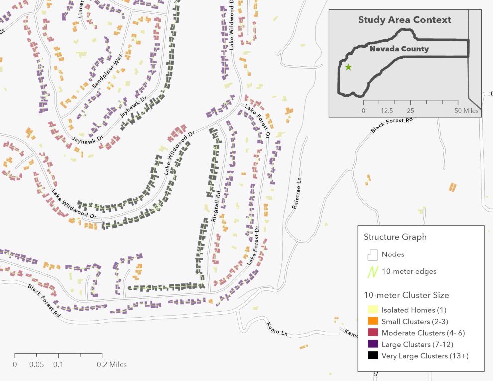
Figure 2. Structure clusters at 10 meters at the neighborhood-scale. This map shows groups of homes close enough to one another (≤10 meters) for direct flame contact to be possible under strong wind conditions. Most structures in this WUI neighborhood are isolated or part of small clusters, but a handful of tightly spaced blocks form larger groups that behave as units during extreme fire events. These patterns highlight where collective hardening and defensible space treatments can provide the greatest benefit. Map by Vibrant Planet Data Commons
At a 10 meter threshold, we can go further by highlighting groups of structures that are close enough for direct flame contact under strong wind conditions (Figure 2). These clusters behave as units. Research consistently shows that home hardening, particularly ember-resistant construction and near-home fuel reduction, substantially increases structure survival during wildfire events.13,14,15 Studies also demonstrate that outcomes improve when many homes in a neighborhood adopt these measures, rather than a few acting alone.16,17
Viewed in that context, large, tightly connected clusters (e.g. <= 10 meter) point to places where collective mitigation may matter most. In other words, hardening a single home within a dense cluster is likely less effective than hardening the cluster together. For communities working with limited mitigation budgets, the Structure Graph helps identify where coordinated home-hardening and defensible-space investments could provide the greatest neighborhood-scale benefit.
Seeing neighborhood-scale exposure pathways
Urban conflagrations often involve more than direct flame contact. Embers lofted from ignited structures can expose buildings well beyond immediate neighbors, motivating analysis at broader distances such as the 50–100 meter structure network. This is where a broader view of neighborhood-scale connectivity, provides a wider lens on potential exposure pathways once fire enters the built environment.
For example, when we color structures by their 100-meter centrality in Nevada County (Figure 3), high-centrality structures stand out immediately. These are not necessarily the homes at the wildland edge; they are the homes most connected to other homes. They represent locations embedded in dense connectivity where exposure could cascade to many nearby structures once ignition occurs.
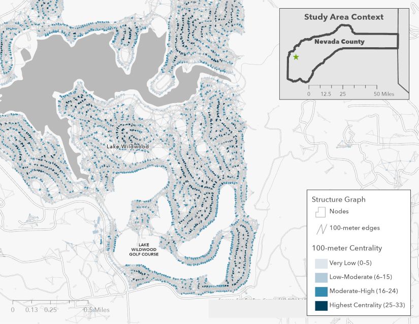
Figure 3. Neighborhood-scale structure connectivity in Nevada County (100m view). This map shows structures colored by degree centrality—the count of nearby structures within a 100-meter network. Higher-centrality structures (darker blue) are embedded within dense, highly interconnected neighborhoods where multiple potential exposure pathways exist. Map by Vibrant Planet Data Commons
Important caveat on directionality: The Structure Graph represents omnidirectional spatial relationships between structures. While fire spread is strongly influenced by wind direction and weather, these factors are not encoded in the graph. As a result, not all connections should be interpreted as equally likely transmission routes. The dataset is best understood as an exposure and connectivity framework that can be combined with directional fire behavior models where appropriate.
From exposure characteristics to modeled outcomes
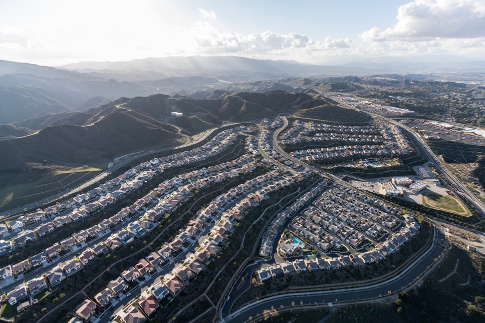
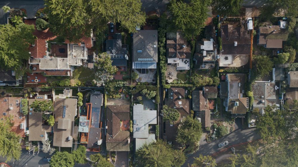
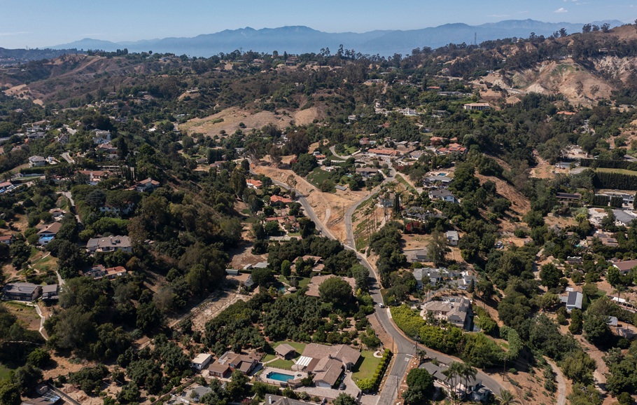
A California wildland–urban interface community viewed from above. Dense suburban form illustrates latent built-environment connectivity common across California’s expanding WUI suburbs. When combined with wildland exposure, small structure separation distances and high neighborhood-scale connectivity help explain why losses may cascade once fire reaches the built environment.
To understand how much this connectivity matters in practice, Vibrant Planet combined structure-graph metrics with structure separation distance and wildland exposure in a machine learning model trained on CAL FIRE’s Damage Inspection (DINS) dataset—the most comprehensive wildfire loss database in the world. The results are intuitive but important:
Homes with high wildland exposure, very small structure separation distances, and high centrality (at 100m) had the highest probability of loss, assuming exposure.
It’s important to note that this does not make the Structure Graph a vulnerability score, nor a predictor of fire behavior. But, it does show that the built-environment patterns captured in the graph offer a meaningful contribution to better understanding and mapping loss outcomes.
From conditional loss to annualized expected loss
Finally, Vibrant Planet aggregated individual probability-of-loss estimates and weighted them by annual burn probability outputs from Pyrologix to create an annualized expected loss surface for Nevada County.
Figure 4 reveals key contrasts:
- Grass Valley shows a high conditional probability of loss, due to its many clusters of tightly packed structures. However, it has a lower annualized expected loss because burn probability is relatively low in the urban core.
- Rural areas to the north, by contrast, have low structure density but high burn probability, resulting in higher annual expected loss despite lower connectivity.
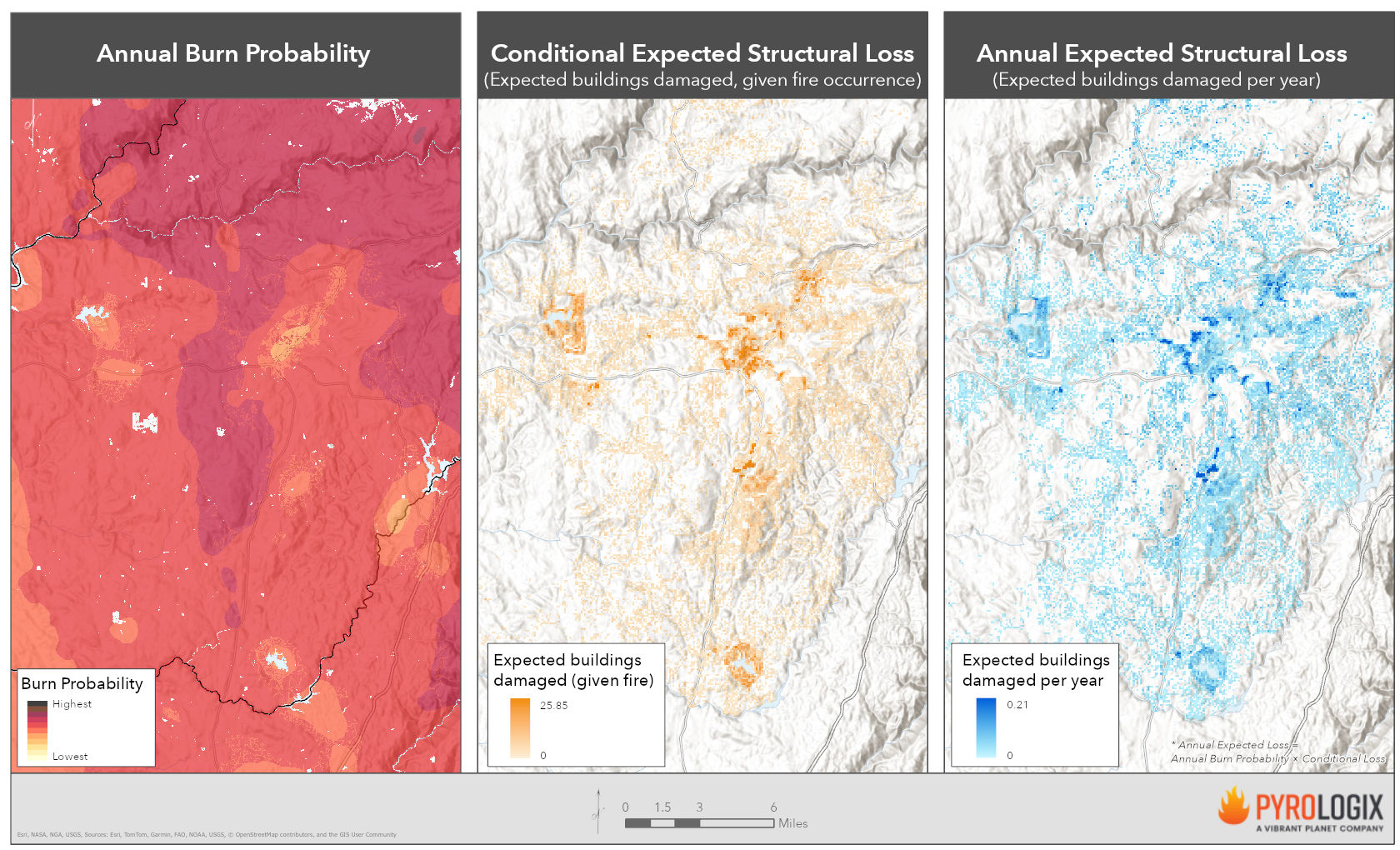
Figure 4. From conditional loss to annual expected structural loss in Nevada County, California.
Left: Annual burn probability from Pyrologix, representing the likelihood that wildfire will burn a given location in any year. Middle: Conditional expected structural loss, calculated by aggregating individual probabilities of loss given wildfire exposure and summarized to 120-meter pixels. Values represent the expected count of buildings damaged, assuming a fire occurs. Right: Annual expected structural loss, calculated by weighting conditional expected loss by annual burn probability. Values represent the expected number of buildings damaged per year. Data and analysis by Pyrologix. Map by Vibrant Planet Data Commons.
Put simply: both wildland exposure and built-environment connectivity shape outcomes, and each matters differently depending on context.
looking ahead
The California Structure Graph is not an endpoint, but a foundational dataset supporting a new generation of built-environment wildfire analysis tools.
Vibrant Planet and partners are already integrating this dataset into upcoming projects that explicitly address structure-to-structure exposure and loss, including structure risk modeling efforts that combine built-environment connectivity with wildland fire exposure, burn probability, and treatment scenarios. By embedding structure graph metrics into broader risk frameworks, these projects move beyond asking whether fire will reach a community to evaluating how losses may cascade once it does.
In the near term, this data will support:
- Structure risk and loss modeling, where connectivity and structure separation distance help explain why some neighborhoods experience cascading losses while others do not.
- Treatment effectiveness and mitigation planning, identifying where fuels treatments, home hardening, or neighborhood-scale interventions are most likely to disrupt high-connectivity fire pathways.
- Community-scale planning and prioritization, helping agencies and planners compare built-environment exposure patterns across regions using a consistent, statewide baseline.
Longer term, the Structure Graph provides a reusable framework that can be extended beyond California. Because it is built from open structure footprints and reproducible methods, the same approach can be applied to other fire-prone states and regions, enabling cross-regional comparison and shared learning around community design and wildfire resilience.
By making this dataset openly available, Vibrant Planet Data Commons works to accelerate collaboration across researchers, practitioners, agencies, and communities—so that insights about structure-to-structure fire dynamics can move more quickly from analysis into action.

Explore the Data Behind the Story
Take a deeper dive into the patterns and trends shaping wildfire behavior across the U.S. Access the full datasets to analyze fire frequency, severity, and historical shifts in fire activity. Whether you're a researcher, land manager, or policymaker, this data provides the foundation for informed decision-making and action.
References
1. Balch, J. K., Iglesias, V., Mahood, A. L., Cook, M. C., Amaral, C., DeCastro, A., Leyk, S., McIntosh, T. L., Nagy, R. C., St. Denis, L. & Tuff, T. The fastest-growing and most destructive fires in the US (2001 to 2020). Science 386, 425–431 (2024).
2. Higuera, P. E., Cook, M. C., Balch, J. K., Stavros, E. N., Mahood, A. L. & St. Denis, L. A. Shifting social-ecological fire regimes explain increasing structure loss from Western wildfires. PNAS Nexus 2, pgad005 (2023). https://doi.org/10.1073/pnas.250588612
3. Thompson, M. P., Calkin, D. E., MacGregor, D. M., Young, B. A., Barrett, K., Fischer, E. C. & Johnson, J. V. Wildfires have created instability within risk transfer markets. Here’s a path forward. Proceedings of the National Academy of Sciences 122, e2530050122 (2025).
4. Radeloff, V. C., Mockrin, M. H., Helmers, D., Carlson, A., Hawbaker, T. J., Martinuzzi, S., Schug, F., Alexandre, P. M., Kramer, H. A. & Pidgeon, A. M. Rising wildfire risk to houses in the United States, especially in grasslands and shrublands. Science 382, 702–707 (2023).
5. Mahmoud, H. & Chulahwat, A. (2018). Unraveling the complexity of wildland–urban interface fires. Scientific Reports, 8, 9315. https://doi.org/10.1038/s41598-018-27215-5
6. Maranghides, A., Link, E., Nazare, S., Hawks, S., McDougald, J., Quarles, S. & Gorham, D. WUI Structure/Parcel/Community Fire Hazard Mitigation Methodology, NIST Technical Note 2205. National Institute of Standards and Technology, Gaithersburg, MD (2022). https://doi.org/10.6028/NIST.TN.2205
7. Zamanialaei, M., San Martin, D., Theodori, M., Purnomo, D. M., Tohidi, A., Lautenberger, C., Qin, Y., Trouvé, A. & Gollner, M. Fire risk to structures in California’s Wildland–Urban Interface. Nature Communications 16, 1–13 (2025). https://doi.org/10.1038/s41467-025-63386-2
8. Insurance Institute for Business & Home Safety. Wildfire Prepared Neighborhood Technical Standard (2025). Available at: https://wildfireprepared.org/wp-content/uploads/Wildfire-Prepared-Neighborhood-Standard-2025.pdf
9. AghaKouchak, A., Chiang, F.-C., Hain, C., Mi, X., Teixeira, J., & Anderson, E. Fire-weather extremes are increasing across the western United States. Nature Computational Science 4, 848–855 (2024). https://doi.org/10.1038/s43588-024-00619-2
10. USDA Forest Service. Wildfire Risk to Communities: Explore your wildfire risk (interactive web application). Wildfire Risk to Communities. https://apps.wildfirerisk.org/explore/overview/06/06057/ (accessed December 15,2025).
11. Los Angeles County. Eaton Fire Recovery. LA County Recovery. https://recovery.lacounty.gov/eaton-fire/ (accessed December 15,2025).
12. Los Angeles County. Palisades Fire Recovery. LA County Recovery. https://recovery.lacounty.gov/palisades-fire/ (accessed December 15,2025).
13. Syphard, A. D., Keeley, J. E., Bar Massada, A., Brennan, T. J. & Radeloff, V. C. Housing arrangement and location influence wildfire structure loss. International Journal of Wildland Fire 21, 215–225 (2012).
14. Quarles, S. L., Valachovic, Y., Nakamura, G. M., Nader, G. A. & de Lasaux, M. Home survival in wildfire-prone areas: Building materials and design considerations. University of California Agriculture & Natural Resources (2010). https://anrcatalog.ucanr.edu/pdf/8393.pdf
15. Manzello, S. L., Foote, E., Maranghides, A., et al. Embers and their role in the wildland–urban interface fire problem. Fire Safety Journal 91, 83–92 (2018). https://doi.org/10.1016/j.firesaf.2017.02.003
16. Insurance Institute for Business & Home Safety (IBHS). Wildfire Prepared Neighborhood: Technical Standard, Version 2025 (2025). Available at https://wildfireprepared.org/wp-content/uploads/Wildfire-Prepared-Neighborhood-Standard-2025.pdf (accessed December 15,2025)
17. Zamanialaei, M., San Martin, D., Theodori, M., Purnomo, D. M., Tohidi, A., Lautenberger, C., Qin, Y., Trouvé, A. & Gollner, M. Fire risk to structures in California’s wildland–urban interface. Nature Communications 16, 1–13 (2025). https://doi.org/10.1038/s41467-025-63386-2